Welcome to CRIKit’s documentation!#

Tutorial can be found here: tutorial.

Core documentation is here: CRIKit core.

API Reference can be found here: crikit API reference.

Documentation on work on extending Pyadjoint is found here: API and description.

Table of contents#

Overview#

CRIKit integrates FEniCS and Pyadjoint with machine learning libraries like JAX and TensorFlow, and provides tools to infer physically-compatible constitutive relations from sparse, noisy observations of a system modeled by partial differential equations. CRIKit bridges the FEniCS world with those of JAX and TensorFlow by storing covering maps between abstract Space classes that represent spaces like a FEniCS FunctionSpace or a space of JAX arrays of a particular shape, or a direct sum of multiple Spaces.

data-flow

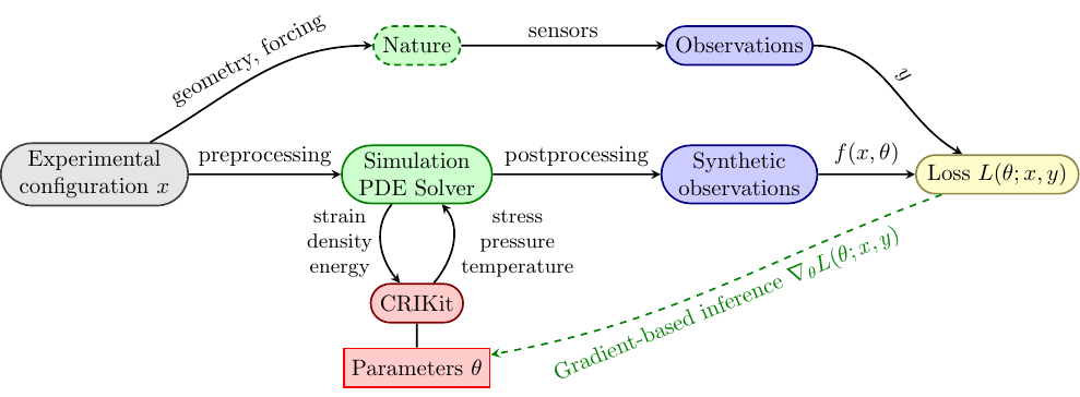
CRIKit also provides tools to help perform post-processing, such as observation operators, as well as a collection of loss functions.

Installation#

See https://gitlab.com/crikit/crikit/#installation for instructions on installing FEniCS. The latest CRIKit release can be installed with

pip install crikit

or, to install the latest development version of CRIKit, you can run

pip install git+https://gitlab.com/crikit/crikit.git

Make sure you install CRIKit into an environment with a working FEniCS installation available, or else the build might fail.

Quick Start#

Constructing And Optimizing a CR#

This guide will show you the basics of constructing and optimizing a simple CR that represents linear elasticity, assuming that you’re already familiar with the basics of the CRIKit finite element backend of your choice, be it FEniCS or [Firedrake]. You can compare the mechanics of CRIKit to that of FEniCS directly by comparing this example to the 2D linear elasticity example from Numerical tours of Computational Mechanics using FEniCS. The primary difference between the model shown here and the linked example in the previous sentence is that here we use a geometrically nonlinear model, as described in the documentation for the libCEED hyperelasticity example.

from crikit import *
import jax
from jax import numpy as jnp
import numpy as np

# set up mesh, FunctionSpace, etc
fe_order = 2
dims = 2
Nx, Ny = 50, 5
L = 20.
H = 1.
mesh = RectangleMesh(Point(0., 0.), Point(L, H), Nx, Ny)
V = VectorFunctionSpace(mesh, "CG", fe_order)
quad_params = {'quadrature_degree' : fe_order + 1}
set_default_covering_params(domain=mesh.ufl_domain(),
                            quad_params=quad_params)
u = Function(V)

def left_boundary(x, on_boundary):
    return near(x[0], 0.)

bcs = [DirichletBC(V, Constant((0., 0.)), left_boundary)]

# these will tell CRIKit what the inputs and ouputs to the CR
# are so that we can automatically generate the scalar and form-invariants
# Let's suppose you want the Cauchy stress tensor as a function of the
# strain sym(grad(u))
input_types = (TensorType.make_symmetric(2, dims, 'strain'),)
output_type = TensorType.make_symmetric(2, dims, 'stress')

# initial guess of parameters
Youngs = 1.0e5
Poisson = 0.3

lmbda = (Youngs * Poisson) / ((1 + Poisson) * (1 - 2 * Poisson))
mu = Youngs / (2 * (1 + Poisson))
# since this is 2-d, we need to use a modified version of lambda
# to make our initial guesses physical
lmbda = 2 * lmbda * mu / (lmbda + 2 * mu)

theta = array([lmbda, mu])

def cr_func(invariants, theta):
    lmbda, mu = theta
    return jnp.array([lmbda * jnp.log1p(invariants[0]), 2 * mu])

cr = CR(output_type, input_types, cr_func, params=[theta])


# If you're in a Jupyter notebook, run this at the bottom of a cell instead of
# calling `print()` on it to get neatly-rendered HTML output.
# This function shows you a description of the scalar and form invariants of `cr`
# in the order they are placed in the arrays
print(cr.invariant_descriptions())

# set the default covering params for crikit.covering so we can automatically
# generate covering maps between spaces of FEniCS Functions and JAX arrays
# Let's just pretend that degree 3 is sufficient quadrature for whatever problem
# we're solving
quad_params = {'quadrature_degree' : 3}
set_default_covering_params(domain=mesh.ufl_domain(), quad_params=quad_params)

# create_ufl_standins() returns a tuple of objects that can act as standins
# for the output of a CR. You can't directly call the CR on the inputs because
# the CR expects JAX arrays as an input, not a FEniCS Function. You'll instead have
# to assembly the variational form F using assemble_with_cr(), which will generate
# a covering map from the space of FEniCS Functions to the space of JAX arrays
# using crikit.covering (and likewise from the output JAX array space to a space of
# `crikit.fe.Function`s), use it to get appropriate arguments, call the CR, and project the result
# back into a Function
target_shape = tuple(i for i in cr.target.shape() if i != -1)

standin_sigma, = create_ufl_standins((target_shape,))

# create your form as if standin_sigma were (cr(sym(grad(u)))
v = TestFunction(V)
# external force
f = Constant((0,-1e-3), name='force')
F = inner(standin_sigma, sym(grad(v))) * dx - inner(f, v) * dx

# define a new sub-tape that records the actions of this equation
with push_tape():
     # a function that we can assemble the variational form into
     # using the `tensor` kwarg of `crikit.assemble()`, which
     # is directly passed on to `crikit.fe.backend.assemble()` 
     # (e.g. `fenics.assemble()`)
     residual = Function(V)

     # input to the CR is sym(grad(u))
     assemble_with_cr(F, cr, sym(grad(u)), standin_sigma, tensor=residual,
     		      quad_params=quad_params)
     ucontrol = Control(u)
     # a ReducedFunction to represent the residual as a function of `u`
     res_rf = ReducedFunction(residual, ucontrol)

# an object to represent the equation defined above
red_eq = ReducedEquation(res_rf, bcs, homogenize_bcs(bcs))

# and an object to solve it. Make sure your .petscrc is set appropriately!
# if you want to pass an assembled Jacobian, use 'jmat_type' : 'assembled',
# but if you want the solver to instead use the matrix-free Jacobian action,
# pass 'jmat_type' : 'action'
solver = SNESSolver(red_eq, {'jmat_type' : 'assembled'})
pred_u = solver.solve(ucontrol)

# define a loss function and an observer

num_slices = 100
seed = 0
# sliced quadratic Wasserstein distance
loss = SlicedWassersteinDistance(V, num_slices, jax.random.PRNGKey(seed), p=2)

class ObservedSubDomain(SubDomain):
      def inside(self, x, on_boundary):
      	  ... # return appropriate True/False if x is in the observed subdomain or not

# observe only on a given SubDomain
observer = SubdomainObserver(mesh, ObservedSubDomain())

# get your observations from somewhere as a Function in V
obs = ...

err = loss(observer(obs), observer(pred_u))


Jhat = ReducedFunctional(err, Control(theta))

#check the derivative
h = np.random.randn(*theta.shape)
v = array(1.0) # test the adjoint
assert taylor_test(Jhat, theta, h, v=v) >= 1.9

# choose an optimization method
opt_method = 'L-BFGS-B'
optimal_params = minimize(Jhat, method=opt_method)

Indices and tables#

About

CRIKit Core